Hairpin formation: Difference between revisions
Rovigattil (talk | contribs) No edit summary |
|||
| (16 intermediate revisions by 3 users not shown) | |||
| Line 1: | Line 1: | ||
<!--<div style="text-align:center"> | |||
http://kratos.phys.uniroma1.it/hairpin.png | |||
</div>--> | |||
[[Category:Examples]] | [[Category:Examples]] | ||
== Introduction == | == Introduction == | ||
In this example, you will simulate a single strand of length 18 and sequence <tt>GCGTTGCTTCTCCAACGC</tt> at 334 K (~61 | In this example, you will simulate a single strand of length 18 and sequence <tt>GCGTTGCTTCTCCAACGC</tt> at 334 K (~61 °C) in three different ways: | ||
* with a | * with a virtual move Monte Carlo (VMMC) simulation of the sequence-averaged (SA) model. The input file is <tt>input</tt>. | ||
* with | * with a VMMC simulation of the sequence-dependent (SD) model. The input file is <code>input_seq_dep</code>. | ||
* with a | * with a VMMC simulation of the SA model in which two base pairs are connected by mutual traps (i.e. additional attractive interactions between two nucleotides). The input file is <tt>input_trap</tt>. | ||
The traps act between the pairs depicted in blue and red in the sequence G<span style="color:red">C</span><span style="color:blue">G</span>TTGCTTCTCCAA<span style="color:blue">C</span><span style="color:red">G</span>C. The details of the interaction associated to the traps can be changed in the file <tt> | The traps act between the pairs depicted in blue and red in the sequence G<span style="color:red">C</span><span style="color:blue">G</span>TTGCTTCTCCAA<span style="color:blue">C</span><span style="color:red">G</span>C. The details of the interaction associated to the traps can be changed in the file <tt>hairpin_forces.dat</tt>. | ||
This strand, if ''T'' is sufficiently low, tends to form an hairpin with a 6-base long stem and a 6-base long loop. | This strand, if ''T'' is sufficiently low, tends to form an hairpin with a 6-base long stem and a 6-base long loop. | ||
The temperature has been chosen to be close to the melting temperature of such a hairpin in the SA version of the model | The temperature has been chosen to be close to the melting temperature of such a hairpin in the SA version of the model | ||
This document explains how to prepare the | This document explains how to prepare the ''hairpin'' example (see [[#Preparation|Preparation]]) and how to run it ([[#Running|Running]]). Section [[#Results|Results]] contains results and plots extracted from the simulation output. In the following, <tt>$EXEC</tt> refers to the oxDNA executable. | ||
== Preparation == | == Preparation == | ||
The script <tt>run.sh</tt> generates the input files and runs all the three simulations, one after the other. With the default input files, each simulation, lasting <math>10^8</math> steps by default, takes approximately one hour on a modern CPU. The default <tt>run.sh</tt> expects <tt>$EXEC</tt> to be in the <tt>../..</tt> directory. If this is not the case, open <tt>run.sh</tt> and change the | The script <tt>run.sh</tt> generates the input files and runs all the three simulations, one after the other. With the default input files, each simulation, lasting <math>10^8</math> steps by default, takes approximately one hour on a modern CPU. The default <tt>run.sh</tt> expects <tt>$EXEC</tt> to be in the <tt>../../bin</tt> directory . If this is not the case, open <tt>run.sh</tt> and change the variables <tt>CODEDIR</tt> and <tt>$OXDNA_BIN</tt> accordingly. | ||
If you only want to generate the initial configuration, you can issue <tt>./run.sh --generate-only</tt>. Then you can run the simulations by yourself. The generated initial configuration files are <tt>initial.top</tt> (which contains the topology) and <tt>initial.conf</tt> (which contains positions and orientations of the nucleotides). | If you only want to generate the initial configuration, you can issue <tt>./run.sh --generate-only</tt>. Then you can run the simulations by yourself. The generated initial configuration files are <tt>initial.top</tt> (which contains the topology) and <tt>initial.conf</tt> (which contains positions and orientations of the nucleotides). | ||
== Running == | == Running == | ||
In order to run the whole example, it is sufficient to issue the command <tt>./run.sh</tt> (or <tt>bash run.sh</tt>). As described in | In order to run the whole example, it is sufficient to issue the command <tt>./run.sh</tt> (or <tt>bash run.sh</tt>). As described in [[#Preparation|Preparation]], you can generate the initial configuration and then run the simulations by hand. The three simulations, described in [[#Introduction|Introduction]], can be performed issuing <tt>$EXEC input</tt>, where <tt>input</tt> is a text file that specifies the simulation configuration. For this example, three files have been prepared: <tt>inputMD</tt>, <tt>inputMD_seq_dep</tt> and <tt>inputTRAP</tt>. The table below reports all the files associated to each simulations. | ||
{| | {| | ||
| Line 25: | Line 29: | ||
! Input | ! Input | ||
! energy file | ! energy file | ||
! HB energy file | |||
! trajectory file | ! trajectory file | ||
! last configuration file | ! last configuration file | ||
| Line 30: | Line 35: | ||
|- | |- | ||
|SA model | |SA model | ||
| | |input | ||
|energy.dat | |energy.dat | ||
|hb_energy.dat | |||
|trajectory.dat | |trajectory.dat | ||
|last_conf.dat | |last_conf.dat | ||
| Line 37: | Line 43: | ||
|- | |- | ||
|SD model | |SD model | ||
| | |input_seq_dep | ||
|energy_seq_dep.dat | |energy_seq_dep.dat | ||
|hb_energy_seq_dep.dat | |||
|trajectory_seq_dep.dat | |trajectory_seq_dep.dat | ||
|last_conf_seq_dep.dat | |last_conf_seq_dep.dat | ||
| Line 44: | Line 51: | ||
|- | |- | ||
|SA model with traps | |SA model with traps | ||
| | |input_trap | ||
|energy_trap.dat | |energy_trap.dat | ||
|hb_energy_trap.dat | |||
|trajectory_trap.dat | |trajectory_trap.dat | ||
|last_conf_trap.dat | |last_conf_trap.dat | ||
| Line 52: | Line 60: | ||
|} | |} | ||
= Results = | == Results == | ||
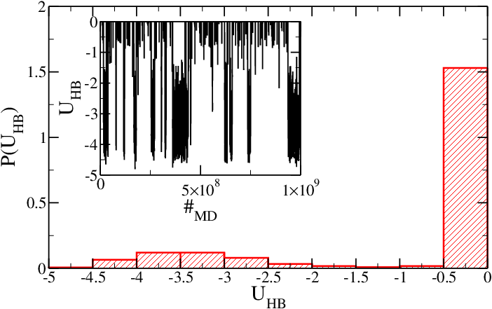
As mentioned in | As mentioned in the [[#Introduction|introduction]], temperature has been chosen so that the hairpin is near its melting temperature when simulated via SA model. Figure 1 shows the probability distribution histogram <math>P(U_{HB})</math> for the hydrogen-bonding (HB) energy <math>U_{HB}</math> of the system (in simulation units). <math>U_{HB}</math> is stored in the second column of the HB energy file as a function of MD steps. Both the minimum in <math>P(U_{HB})</math> and a direct inspection of the time series (inset) show that the hairpin is indeed near the melting temperature, since <math>U_{HB}</math> oscillates between 0 (no HBs) and ~ -3.5, which corresponds to 4-5 hydrogen-bonded nucleotides. At this temperature the fraying effect is relevant, and therefore the last base-pair is not always formed. | ||
<div style="text-align:center"> | |||
[[Image:histo_MD.png]] | |||
<h5>Figure 1: Probability of having a hydrogen-bonding interaction energy <math>U_{HB}</math> for the SA model. Inset: time series of the hydrogen-bonding energy.</h5> | |||
</div> | |||
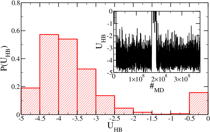
Figure 2 shows <math>P(U_{HB})</math> and <math>U_{HB}</math> for the SD hairpin. In this case, one expects a different melting temperature. Indeed, at this temperature the hairpin is nearly always in its folded conformation and the average value of <math>U_{HB}</math> is lower than in the SA case. Although stacking interactions play a role, the major contribution to this effect is due to the presence of four <tt>GC</tt> only two <tt>AT</tt> base-pairs in the stem. | |||
<div style="text-align:center"> | |||
[[Image:histo_MD_seq_dep.png]] | |||
<h5>Figure 2: Same as Figure 1, but for the SD model.</h5> | |||
</div> | |||
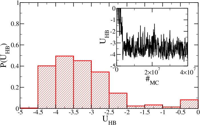
If mutual traps between stem base-pairs are introduced, then the equilibrium properties of the hairpin are changed and, even if the SA model is employed, the hairpin is always (after the initial equilibration) in its folded conformation. The use of mutual traps can highly decrease the simulation time required by the folding of strands into target structures (like DNA origami or DNA constructs). | |||
<div style="text-align:center"> | |||
[[Image:histo_TRAP.png]] | |||
<h5>Figure 3: Same as Figure 1, but for the system with mutual traps. Time is expressed in Monte Carlo sweeps.</h5> | |||
</div> | |||
Latest revision as of 09:24, 18 June 2015
Introduction
In this example, you will simulate a single strand of length 18 and sequence GCGTTGCTTCTCCAACGC at 334 K (~61 °C) in three different ways:
- with a virtual move Monte Carlo (VMMC) simulation of the sequence-averaged (SA) model. The input file is input.
- with a VMMC simulation of the sequence-dependent (SD) model. The input file is
input_seq_dep. - with a VMMC simulation of the SA model in which two base pairs are connected by mutual traps (i.e. additional attractive interactions between two nucleotides). The input file is input_trap.
The traps act between the pairs depicted in blue and red in the sequence GCGTTGCTTCTCCAACGC. The details of the interaction associated to the traps can be changed in the file hairpin_forces.dat.
This strand, if T is sufficiently low, tends to form an hairpin with a 6-base long stem and a 6-base long loop. The temperature has been chosen to be close to the melting temperature of such a hairpin in the SA version of the model
This document explains how to prepare the hairpin example (see Preparation) and how to run it (Running). Section Results contains results and plots extracted from the simulation output. In the following, $EXEC refers to the oxDNA executable.
Preparation
The script run.sh generates the input files and runs all the three simulations, one after the other. With the default input files, each simulation, lasting Failed to parse (SVG (MathML can be enabled via browser plugin): Invalid response ("Math extension cannot connect to Restbase.") from server "https://wikimedia.org/api/rest_v1/":): {\displaystyle 10^8} steps by default, takes approximately one hour on a modern CPU. The default run.sh expects $EXEC to be in the ../../bin directory . If this is not the case, open run.sh and change the variables CODEDIR and $OXDNA_BIN accordingly.
If you only want to generate the initial configuration, you can issue ./run.sh --generate-only. Then you can run the simulations by yourself. The generated initial configuration files are initial.top (which contains the topology) and initial.conf (which contains positions and orientations of the nucleotides).
Running
In order to run the whole example, it is sufficient to issue the command ./run.sh (or bash run.sh). As described in Preparation, you can generate the initial configuration and then run the simulations by hand. The three simulations, described in Introduction, can be performed issuing $EXEC input, where input is a text file that specifies the simulation configuration. For this example, three files have been prepared: inputMD, inputMD_seq_dep and inputTRAP. The table below reports all the files associated to each simulations.
| Type | Input | energy file | HB energy file | trajectory file | last configuration file | log file |
|---|---|---|---|---|---|---|
| SA model | input | energy.dat | hb_energy.dat | trajectory.dat | last_conf.dat | log.dat |
| SD model | input_seq_dep | energy_seq_dep.dat | hb_energy_seq_dep.dat | trajectory_seq_dep.dat | last_conf_seq_dep.dat | log_seq_dep.dat |
| SA model with traps | input_trap | energy_trap.dat | hb_energy_trap.dat | trajectory_trap.dat | last_conf_trap.dat | log_trap.dat |
Results
As mentioned in the introduction, temperature has been chosen so that the hairpin is near its melting temperature when simulated via SA model. Figure 1 shows the probability distribution histogram Failed to parse (SVG (MathML can be enabled via browser plugin): Invalid response ("Math extension cannot connect to Restbase.") from server "https://wikimedia.org/api/rest_v1/":): {\displaystyle P(U_{HB})} for the hydrogen-bonding (HB) energy Failed to parse (SVG (MathML can be enabled via browser plugin): Invalid response ("Math extension cannot connect to Restbase.") from server "https://wikimedia.org/api/rest_v1/":): {\displaystyle U_{HB}} of the system (in simulation units). Failed to parse (SVG (MathML can be enabled via browser plugin): Invalid response ("Math extension cannot connect to Restbase.") from server "https://wikimedia.org/api/rest_v1/":): {\displaystyle U_{HB}} is stored in the second column of the HB energy file as a function of MD steps. Both the minimum in Failed to parse (SVG (MathML can be enabled via browser plugin): Invalid response ("Math extension cannot connect to Restbase.") from server "https://wikimedia.org/api/rest_v1/":): {\displaystyle P(U_{HB})} and a direct inspection of the time series (inset) show that the hairpin is indeed near the melting temperature, since Failed to parse (SVG (MathML can be enabled via browser plugin): Invalid response ("Math extension cannot connect to Restbase.") from server "https://wikimedia.org/api/rest_v1/":): {\displaystyle U_{HB}} oscillates between 0 (no HBs) and ~ -3.5, which corresponds to 4-5 hydrogen-bonded nucleotides. At this temperature the fraying effect is relevant, and therefore the last base-pair is not always formed.
Figure 1: Probability of having a hydrogen-bonding interaction energy Failed to parse (SVG (MathML can be enabled via browser plugin): Invalid response ("Math extension cannot connect to Restbase.") from server "https://wikimedia.org/api/rest_v1/":): {\displaystyle U_{HB}} for the SA model. Inset: time series of the hydrogen-bonding energy.
Figure 2 shows Failed to parse (SVG (MathML can be enabled via browser plugin): Invalid response ("Math extension cannot connect to Restbase.") from server "https://wikimedia.org/api/rest_v1/":): {\displaystyle P(U_{HB})}
and Failed to parse (SVG (MathML can be enabled via browser plugin): Invalid response ("Math extension cannot connect to Restbase.") from server "https://wikimedia.org/api/rest_v1/":): {\displaystyle U_{HB}}
for the SD hairpin. In this case, one expects a different melting temperature. Indeed, at this temperature the hairpin is nearly always in its folded conformation and the average value of Failed to parse (SVG (MathML can be enabled via browser plugin): Invalid response ("Math extension cannot connect to Restbase.") from server "https://wikimedia.org/api/rest_v1/":): {\displaystyle U_{HB}}
is lower than in the SA case. Although stacking interactions play a role, the major contribution to this effect is due to the presence of four GC only two AT base-pairs in the stem.
If mutual traps between stem base-pairs are introduced, then the equilibrium properties of the hairpin are changed and, even if the SA model is employed, the hairpin is always (after the initial equilibration) in its folded conformation. The use of mutual traps can highly decrease the simulation time required by the folding of strands into target structures (like DNA origami or DNA constructs).


